Module 4 - Crime Analysis
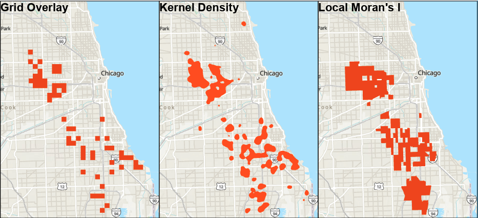 |
| Comparison of Crime Analysis Methods |
The Chicago crime hotspot map that appears best for predicting future homicides would likely be the Grid Overlay. This is because the crime density was highest within this technique, meaning it was the best predictor of 2018 crimes by capturing the most crimes within its area. This is despite having the smallest hotspot area out of the three analysis techniques. Larger hotspot areas are not necessarily beneficial to allocating resources, as larger areas will always contain more crimes and will thus be somewhat meaningless and too encompassing. Thus, I believe the Grid Overlay was the best predictor as it was the most precise and accurate out of the three techniques.
Now I will describe the methods I took in conducting the three types of analyses
Now I will describe the methods I took in conducting the three types of analyses
Grid Overlay
First, I utilized the Spatial Join tool to join the attributes of the grid cells and 2017 homicide layers. I used the Select by Attributes tool to select the grids that contained 1 or more homicides in 2017. For this tool, I used the newly joined layer as the input and the join_count field is greater than 0 as my parameters. Then, I located the total number of attributes on the bottom left of the attribute table and divided this number by 5 to determine how many attributes should be in each quintile. I sorted the attribute table by the Join_Count field and then manually selected this number of attributes from the table. I then exported my selections as a new shapefile by right clicking the layer and clicking export selection to new layer. I then used the dissolve tool with the newly created DISSOLVE field in the attribute table to create the multipart feature map that could be used for further analysis.
Kernel Density
I used the Kernel Density tool with the specified parameters in the lab instructions to create a kernel density layer of the 2017 homicides in Chicago. I used the statistics option in the attribute table to locate the mean value, and then performed manual calculations on this value to determine what the breaks in the data should be. These breaks were updated in the symbology of the newly created kernel layer, and then I used the Reclassify tool to assign new values to the different breaks. I then used the Raster to Polygon tool so that I could run the Select by Attributes tool to select and export the values of 2 (aka the areas with more crime).
Local Moran’s I
For this analysis, I also used the Spatial Join tool to combine the census tracts and 2017 homicides. After opening up the newly created attribute table, I added a field that I would use to calculate the crime rate for each tract. Then I used the Calculate Field tool and crimes/housing units*1000 to determine the crime density for each tract. This tool automatically populated the crime density field that was added to the attribute table. I then used the Cluster and Outlier Analysis (Anselin Local Moran’s I) tool with the spatially joined layer and the crime rates as the input fields. I used an SQL theory within the Select by Attributes tool to select only those outputs that had high levels of crime and then used the Dissolve tool with the Dissolve by COType IDW field input to create one, single multipart layer for later analysis.
 |
| Washington DC Burglary Rates |
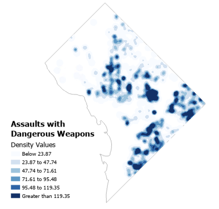 |
| Washington DC Assault Densities |